SQL Server POLYFIT_q Function
Updated 2024-03-06 21:31:27.857000
Description
Use the table-valued function POLYFIT_q for calculating the coefficients of a polynomial p(x) of degree n that fits the x- and y-values supplied to the function. The result is a two-column table having n+1 rows, containing the polynomial coefficients in descending powers:
y=p_1x^n+p_2x^{n-1}+\dots+p_nx^1+p_{n+1}x^0
POLYFIT_q only calculates the coefficients of the polynomial. To evaluate the polynomial for a value of x, use the POLYVAL function.
Syntax
SELECT * FROM [westclintech].[wct].[POLYFIT_q](
  <@XY_RangeQuery, nvarchar(max),>
 ,<@n, int,>)
Arguments
@XY_RangeQuery
the SELECT statement, as text, used to determine the x- and y-values to be evaluated. The SELECT statement specifies the column names from the table or view or can be used to enter the x- and y-values directly. Data returned from the @XY_RangeQuery select must be of the type float or of a type that implicitly converts to float.
@n
an integer specifying the degree of the polynomial.
Return Type
table
{"columns": [{"field": "colName", "headerName": "Name", "header": "name"}, {"field": "colDatatype", "headerName": "Type", "header": "type"}, {"field": "colDesc", "headerName": "Description", "header": "description", "minWidth": 1000}], "rows": [{"id": "8a955e64-d637-47cf-bd72-3521bfec874f", "colName": "coe_num", "colDatatype": "int", "colDesc": "The index-number of the coeeficient"}, {"id": "56957589-b1a6-4fe1-ae75-c02189383f29", "colName": "coe_val", "colDatatype": "int", "colDesc": "The value of the coefficient"}]}
Remarks
The x- and y-values are passed to the function as pairs
If x is NULL or y is NULL, the pair is not used in the calculation.
@n must be less than or equal to the number of rows returned by @XY_RangeQuery
Use the POLYFIT function for simpler queries.
Use the POLYVAL function to evaluate the polynomial for an x-value.
Examples
In this example, we will use the SeriesFloat function to generate a series of x-values equally spaced in the interval [0, 2.5] and then evaluate the error function, ERF, at those points.
SELECT SeriesValue as x,
       wct.ERF(SeriesValue) as y
from wct.SeriesFloat(0, 2.5, 0.1, NULL, NULL);
Since the function will execute the @XY_RangeQuery, all we need to do is put single quotes around the previous statement and pass it into POLYFIT_q . We will specify an approximating polynomial of 6 degrees.
SET NOCOUNT ON;
SELECT *
FROM wct.POLYFIT_q(
                      'SELECT SeriesValue as x
      ,wct.ERF(SeriesValue) as y
      from wct.SeriesFloat(0,2.5,0.1,NULL,NULL)'
                ,
                      --@XY_RangeQuery
                      6 --@n
                  );
This produces the following result.
{"columns":[{"field":"coe_num","headerClass":"ag-right-aligned-header","cellClass":"ag-right-aligned-cell"},{"field":"coe_val","headerClass":"ag-right-aligned-header","cellClass":"ag-right-aligned-cell"}],"rows":[{"coe_num":"7","coe_val":"0.000441173957975313"},{"coe_num":"6","coe_val":"1.10644604471276"},{"coe_num":"5","coe_val":"0.147104056213985"},{"coe_num":"4","coe_val":"-0.743462848525445"},{"coe_num":"3","coe_val":"0.421736169319562"},{"coe_num":"2","coe_val":"-0.0982995751931375"},{"coe_num":"1","coe_val":"0.00841937176047103"}]}
This means that there are 7 coefficients. We could run the following SQL to see the structure of the approximating polynomial.
SELECT *
  FROM wct.POLYFIT_q(
           'SELECT SeriesValue as x
      ,wct.ERF(SeriesValue) as y
      from wct.SeriesFloat(0,2.5,0.1,NULL,NULL)'                                                                                 ,
           --@XY_RangeQuery
           6--@n
    )
This produces the following result.
{"columns":[{"field":"coe_num","headerClass":"ag-right-aligned-header","cellClass":"ag-right-aligned-cell"},{"field":"coe_val","headerClass":"ag-right-aligned-header","cellClass":"ag-right-aligned-cell"},{"field":"pow","headerClass":"ag-right-aligned-header","cellClass":"ag-right-aligned-cell"}],"rows":[{"coe_num":"7","coe_val":"0.000441173957975313","pow":"0"},{"coe_num":"6","coe_val":"1.10644604471276","pow":"1"},{"coe_num":"5","coe_val":"0.147104056213985","pow":"2"},{"coe_num":"4","coe_val":"-0.743462848525445","pow":"3"},{"coe_num":"3","coe_val":"0.421736169319562","pow":"4"},{"coe_num":"2","coe_val":"-0.0982995751931375","pow":"5"},{"coe_num":"1","coe_val":"0.00841937176047103","pow":"6"}]}
Thus, the approximating polynomial would be:
0.00841937x6 - 0.0982996x5 + 0.421736x 4 - 0.743463x3 + 0.147104x 2 + 1.10645x + 0.000441174
We can inspect the fit of the approximating polynomial by creating a table of the x- and y-values and evaluating the approximating polynomial for each x and comparing it to the actual y-values. While we could do this using the output of the POLYFIT_q table-valued function, it is much simpler to just use the POLYVAL function.
SET NOCOUNT ON;
SELECT SeriesValue as x,
       wct.ERF(SeriesValue) as y
INTO #erf
FROM wct.SeriesFloat(0, 2.5, 0.1, NULL, NULL);
SELECT a.x,
       ROUND(a.y, 8) as y,
       ROUND(wct.POLYVAL(b.x, b.y, 6, a.x), 8) as f,
       ROUND(wct.POLYVAL(b.x, b.y, 6, a.x) - a.y, 8) as [f - y]
FROM #erf a,
     #erf b
GROUP BY a.x,
         a.y
ORDER BY 1;
DROP TABLE #erf;
This produces the following result.
{"columns":[{"field":"x","headerClass":"ag-right-aligned-header","cellClass":"ag-right-aligned-cell"},{"field":"y","headerClass":"ag-right-aligned-header","cellClass":"ag-right-aligned-cell"},{"field":"f","headerClass":"ag-right-aligned-header","cellClass":"ag-right-aligned-cell"},{"field":"f - y","headerClass":"ag-right-aligned-header","cellClass":"ag-right-aligned-cell"}],"rows":[{"x":"0","y":"0","f":"0.00044117","f - y":"0.00044117"},{"x":"0.1","y":"0.11246292","f":"0.11185456","f - y":"-0.00060836"},{"x":"0.2","y":"0.22270259","f":"0.2223107","f - y":"-0.00039189"},{"x":"0.3","y":"0.32862676","f":"0.32872419","f - y":"9.743E-05"},{"x":"0.4","y":"0.42839236","f":"0.42879896","f - y":"0.00040661"},{"x":"0.5","y":"0.52049988","f":"0.52092556","f - y":"0.00042568"},{"x":"0.6","y":"0.60385609","f":"0.60408433","f - y":"0.00022824"},{"x":"0.7","y":"0.67780119","f":"0.67775481","f - y":"-4.638E-05"},{"x":"0.8","y":"0.74210096","f":"0.74183105","f - y":"-0.00026992"},{"x":"0.9","y":"0.79690821","f":"0.79654307","f - y":"-0.00036515"},{"x":"1","y":"0.84270079","f":"0.84238439","f - y":"-0.0003164"},{"x":"1.1","y":"0.88020507","f":"0.88004559","f - y":"-0.00015948"},{"x":"1.2","y":"0.91031398","f":"0.9103539","f - y":"3.992E-05"},{"x":"1.3","y":"0.93400794","f":"0.93421894","f - y":"0.00021099"},{"x":"1.4","y":"0.95228512","f":"0.95258445","f - y":"0.00029933"},{"x":"1.5","y":"0.96610515","f":"0.96638612","f - y":"0.00028097"},{"x":"1.6","y":"0.97634838","f":"0.97651543","f - y":"0.00016704"},{"x":"1.7","y":"0.98379046","f":"0.98378962","f - y":"-8.3E-07"},{"x":"1.8","y":"0.9890905","f":"0.98892772","f - y":"-0.00016279"},{"x":"1.9","y":"0.99279043","f":"0.99253252","f - y":"-0.00025791"},{"x":"2","y":"0.99532227","f":"0.9950788","f - y":"-0.00024347"},{"x":"2.1","y":"0.99702053","f":"0.99690743","f - y":"-0.0001131"},{"x":"2.2","y":"0.99813715","f":"0.9982257","f - y":"8.855E-05"},{"x":"2.3","y":"0.99885682","f":"0.99911355","f - y":"0.00025673"},{"x":"2.4","y":"0.99931149","f":"0.99953599","f - y":"0.00022451"},{"x":"2.5","y":"0.99959305","f":"0.99936154","f - y":"-0.00023151"}]}
It looks like the approximating polynomial is accurate to about 3 or 4 decimal places. In fact if we graphed the results, they would look like this:
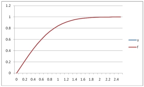
We can see that in this range, [0, 2.5] the fit between the y-values and the f-values is quite good. However, what if we extend the range of the interval from 2.5 to 6? We will simply change SERIESFLOAT to stop at 6.0 rather than 2.5 and then graph the output.
SELECT SeriesValue as x,
       wct.ERF(SeriesValue) as y
INTO #erf
FROM wct.SeriesFloat(0, 6.0, 0.1, NULL, NULL);
SELECT a.x,
       a.y,
       wct.POLYVAL(b.x, b.y, 6, a.x) as f,
       wct.POLYVAL(b.x, b.y, 6, a.x) - a.y as [f - y]
FROM #erf a,
     #erf b
GROUP BY a.x,
         a.y
ORDER BY 1;
This produces the following graph.
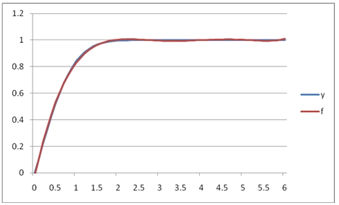
It's important to note that coefficients in the interval [0, 6] are different than the coefficients in the interval [0, 2.5] because there were more x- and y-values passed to the function. What if we wanted to use the coefficients from the [0, 2.5] interval to predict the values in the [0, 6] interval?
SELECT SeriesValue as x,
       wct.ERF(SeriesValue) as y
INTO #erf
FROM wct.SeriesFloat(0, 2.5, 0.1, NULL, NULL);
SELECT SeriesValue as x,
       wct.ERF(SeriesValue) as y,
       wct.POLYVAL(b.x, b.y, 6, a.SeriesValue) as f,
       wct.POLYVAL(b.x, b.y, 6, a.SeriesValue) - wct.ERF(SeriesValue) as [f - y]
FROM wct.SeriesFloat(0, 6.0, 0.1, NULL, NULL) a ,
     #erf b
GROUP BY a.SeriesValue,
         wct.ERF(SeriesValue)
ORDER BY 1;
DROP TABLE #erf;
This produces the following graph.
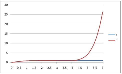
As you can see, the polynomial approximation quickly diverges from the function in the region above 2.5.
Let's look at a different example. In this example we will look at some interest rate values over a time-horizon and calculate the 3rd degree polynomial approximation. The x-values represent the number of years and the y-values are the decimal values of the interest rate (.01 = 1%).
SET NOCOUNT ON;
SELECT *
FROM wct.POLYFIT_q(
                      'SELECT *
from (VALUES
      (1,0.0028),
      (2,0.0056),
      (3,0.0085),
      (5,0.0164),
      (7,0.0235),
      (10,0.0299),
      (20,0.0382),
      (30,0.0406)
      ) n(x,y)',
                      3
                  );
This produces the following result.
{"columns":[{"field":"coe_num","headerClass":"ag-right-aligned-header","cellClass":"ag-right-aligned-cell"},{"field":"coe_val","headerClass":"ag-right-aligned-header","cellClass":"ag-right-aligned-cell"}],"rows":[{"coe_num":"4","coe_val":"-0.00325347316656146"},{"coe_num":"3","coe_val":"0.00497032283231484"},{"coe_num":"2","coe_val":"-0.000198230933179584"},{"coe_num":"1","coe_val":"2.70683303153489E-06"}]}
While we would always recommend using the POLYVAL function to calculate the polynomial approximation for any x-value, in this example we will use the results of the POLYFIT_q TVF to calculate the rates for each year from 1 through 30 out to 4 decimal places.
SET NOCOUNT ON;
SELECT coe_num,
       coe_val,
       ROW_NUMBER() OVER (order by coe_num DESC) - 1 as pow
into #coe
FROM wct.POLYFIT_q(
                      'SELECT *
from (VALUES
      (1,0.0028),
      (2,0.0056),
      (3,0.0085),
      (5,0.0164),
      (7,0.0235),
      (10,0.0299),
      (20,0.0382),
      (30,0.0406)
      ) n(x,y)',
                      3
                  );
SELECT SeriesValue as y,
       ROUND(SUM(POWER(SeriesValue, pow) * coe_val), 4) as r
FROM wct.SeriesInt(1, 30, NULL, NULL, NULL) ,
     #coe
GROUP BY SeriesValue
ORDER BY 1;
DROP TABLE #coe;
This produces the following result.
{"columns":[{"field":"y","headerClass":"ag-right-aligned-header","cellClass":"ag-right-aligned-cell"},{"field":"r","headerClass":"ag-right-aligned-header","cellClass":"ag-right-aligned-cell"}],"rows":[{"y":"1","r":"0.0015"},{"y":"2","r":"0.0059"},{"y":"3","r":"0.0099"},{"y":"4","r":"0.0136"},{"y":"5","r":"0.017"},{"y":"6","r":"0.02"},{"y":"7","r":"0.0228"},{"y":"8","r":"0.0252"},{"y":"9","r":"0.0274"},{"y":"10","r":"0.0293"},{"y":"11","r":"0.031"},{"y":"12","r":"0.0325"},{"y":"13","r":"0.0338"},{"y":"14","r":"0.0349"},{"y":"15","r":"0.0358"},{"y":"16","r":"0.0366"},{"y":"17","r":"0.0373"},{"y":"18","r":"0.0378"},{"y":"19","r":"0.0382"},{"y":"20","r":"0.0385"},{"y":"21","r":"0.0388"},{"y":"22","r":"0.039"},{"y":"23","r":"0.0391"},{"y":"24","r":"0.0393"},{"y":"25","r":"0.0394"},{"y":"26","r":"0.0395"},{"y":"27","r":"0.0397"},{"y":"28","r":"0.0399"},{"y":"29","r":"0.0402"},{"y":"30","r":"0.0405"}]}